#5 1RB1RA_0LC0RF_1LD1LC_1RE1LB_---0RA_1RF0RD: is the erosion deterministically bounded?
Research note, 2026-10-10. Code: research/code/, figures: research/img/.
Answer in four lines
- No deterministic bound was found, and every certificate family tried fails by a factor of 5 to 12 (section 5).
- What the data shows: the edge is a chaotic front moving into the block at a steady 0.039 cells per bounce (constant across four decades, 10^4 to 10^8 bounces). In short windows it can still outrun the block: +149 cells in 128 bounces at worst. Over 10^8 bounces the block never lost more than 47 cells net, and it was never shorter than 33 cells after bounce 40.
- Why simple proofs fail: - What decides a burst sits 50 to 500+ cells deep in the edge. - The edge carries about 0.63 bits of entropy per cell. - Any certificate (potential, regular language) must "see" that deep, and every finite window we tried allows fake cycles that erode at 5 cells per bounce or more.
- Recommendation: treat #5 as cryptid-like for proof purposes and follow the protocol: formalize the rules (done, section 1), flag, stop. Section 8 lists the one route with a real but small chance.
Side result (computer-checked, not a proof): with the exact wall model, the machine does not halt in its first ~9.6·10^15 steps (10^8 bounces).
1. What one bounce is: 7 exact rules
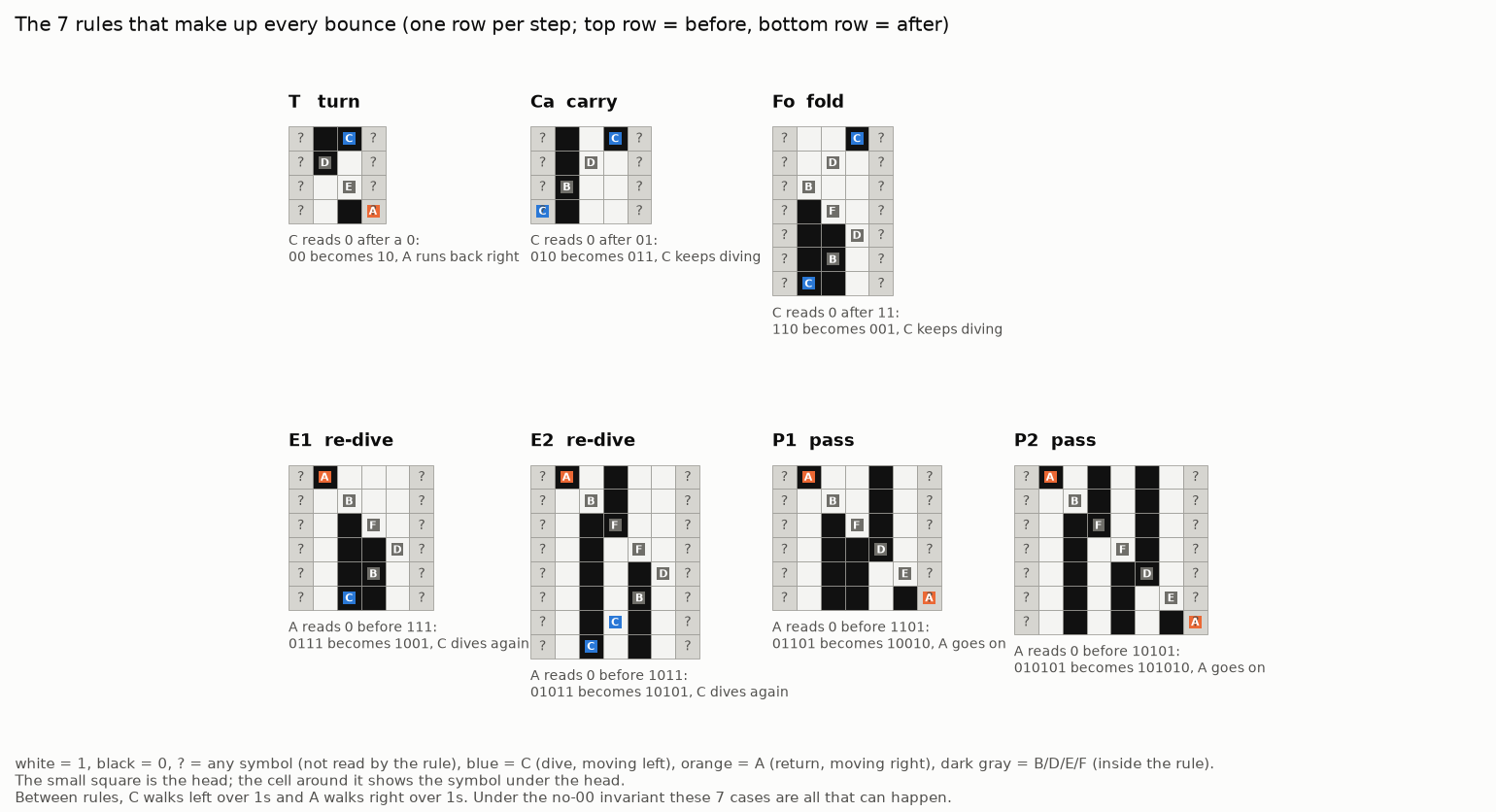
start: constructed, each rule from its own minimal context · rows: every step · window: the cells the rule touches, plus one
?cell on each side · legend: white = 1, black = 0,?= any symbol, blue = C, orange = A, dark gray = B/D/E/F · style: custom
Every bounce, from "C at the edge's last 0" until "A steps onto an untouched block cell", is a sequence of these rules. Between rules, C walks left over 1s and A walks right over 1s.
| rule | before → after (wiki notation) | steps |
|---|---|---|
| T turn | x 0 0 <C y → x 1 0 A> y |
3 |
| Ca carry | x 0 1 0 <C y → x <C 0 1 1 y |
3 |
| Fo fold | x 1 1 0 <C y → x 0 <C 0 1 y |
6 |
| E1 re-dive | x A> 0 1 1 1 y → x 1 0 <C 0 1 y |
5 |
| E2 re-dive | x A> 0 1 0 1 1 y → x 1 0 <C 1 0 1 y |
7 |
| P1 pass | x A> 0 1 1 0 1 y → x 1 0 0 1 0 A> y |
5 |
| P2 pass | x A> 0 1 0 1 0 1 y → x 1 0 1 0 1 0 A> y |
6 |
- Status: proven by case analysis. C reading 0 sees one of the left contexts
0,01or11. A reading 0 sees one of the 4 right contexts above, since the no-00 invariant rules out every other one. Each rule was also checked 60/60 withtools/sim.pyon random x and y (code/verify_rules.py). - Erosion happens only here: E1, E2, P1 or P2 fires where A reaches the edge's last 0 next to the block. E1 and E2 also launch a new dive from the block.
- Reachable fact (empirical): every edge word ends in
010(2,000,000 of 2,000,000 bounces checked). So every bounce opens with Ca.
The dive is a binary-counter carry (exact)
Write the edge as runs of 1s separated by single 0s, with 00 counted as a run of length 0. A dive started at the right end does the following:
runs, right to left:   ...  a(j-4)  a(j-3)  a(j-2)  a(j-1)  a(j) | block
C examines:                  ^               ^               ^
  a odd  -> rewrite "1^a 0" into "1 1 (0 1)^((a-1)/2)", skip the next run, examine the one after it
  a even -> rewrite "0 1^a 0" into "1 0 (0 1)^(a/2)" and turn (A heads right)
This is an increment of a binary counter whose digits are the parities of every other run: odd means digit 1 (carry on), even means digit 0 (stop). It follows from Ca, Fo and T by induction on a, and it matched 15,450 of 15,450 random run sequences (code/divecheck.py).
It matches the ruler pattern of dive depths seen in receding phases: 9, 18, 9, 27, 9, 18, 9, ...
The return pass is not a clean counter. Its E1 and E2 rules re-dive repeatedly (the "tiny wiggles"). The rewrites also change the run structure, so the "digits" do not keep their meaning from one bounce to the next. That mixing is where the chaos comes from.
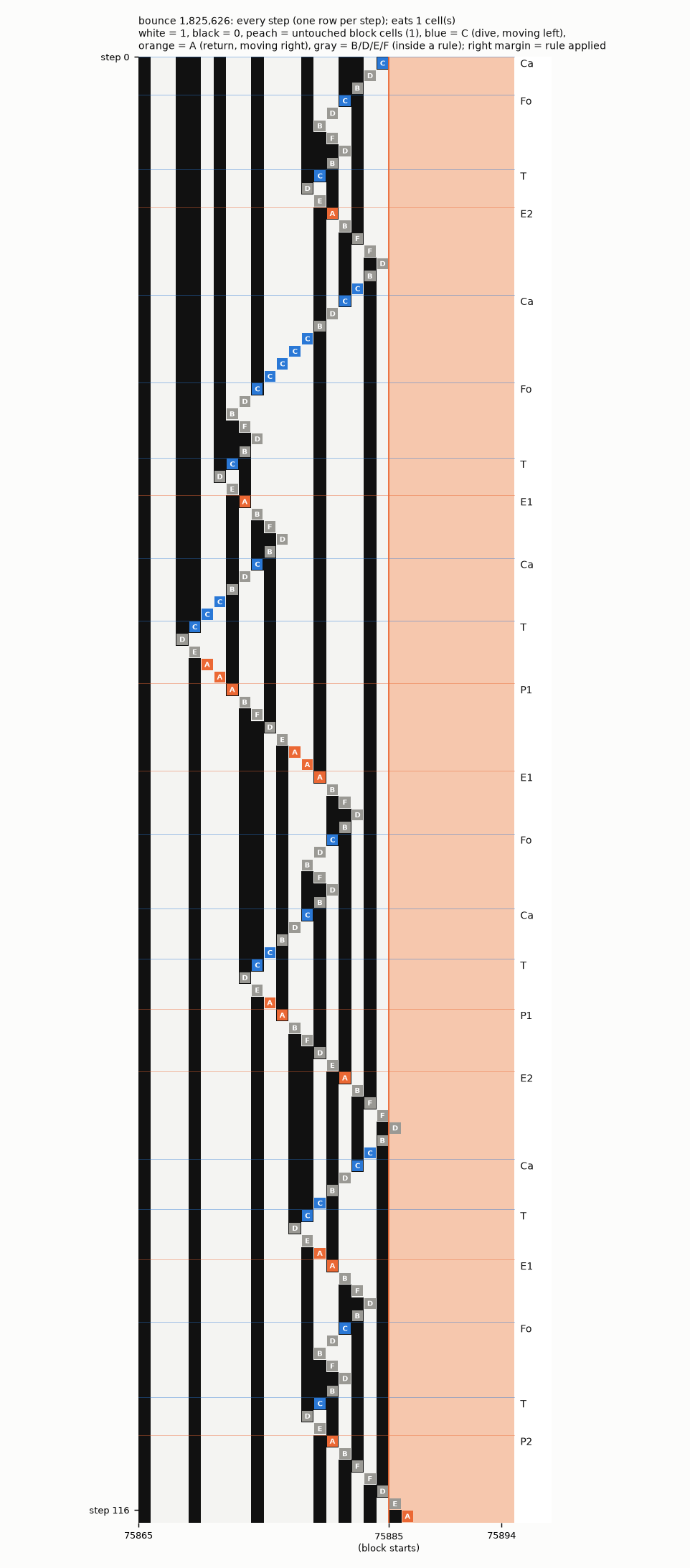
start: mid-run, the tape after bounce 1,825,625 (about 3.2·10^12 steps) · rows: every step of bounce 1,825,626 (117 rows) · window: cells 75,865..75,894, one square per cell · legend: white = 1, black = 0, peach = untouched block 1s, blue = C, orange = A, gray = B/D/E/F; the right margin names the rule applied at that row · style: custom
2. The race: block vs edge
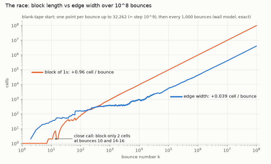
start: blank tape · rows: n/a (a chart): one point per bounce up to bounce 32,262 (= step 10^9, real simulation), then every 1,000 bounces (wall model) · legend: orange = block length n, blue = edge width |w| · style: custom chart
| bounces | 10^3 to 10^4 | 10^4 to 10^5 | 10^5 to 10^6 | 10^6 to 10^7 | 10^7 to 10^8 |
|---|---|---|---|---|---|
| cells eaten per bounce | 0.0566 | 0.0489 | 0.0392 | 0.0388 | 0.0395 |
- Edge width at 10^8 bounces: 3,940,720. The fit is |w| ∝ k^0.995, so the growth is linear.
- Wall-model exactness:
- The bounce map ignores the block length n whenever the head reads at most e+1 block cells. The run reports this every bounce (it never read past cell b+e).
- From bounce 40 on, n ≥ 33 > 15 + 3 (largest e: 15), so the 10^8-bounce run is an exact simulation of the machine.
- It never reached E reading 0.
3. Bursts: the edge can outrun the block, but only briefly
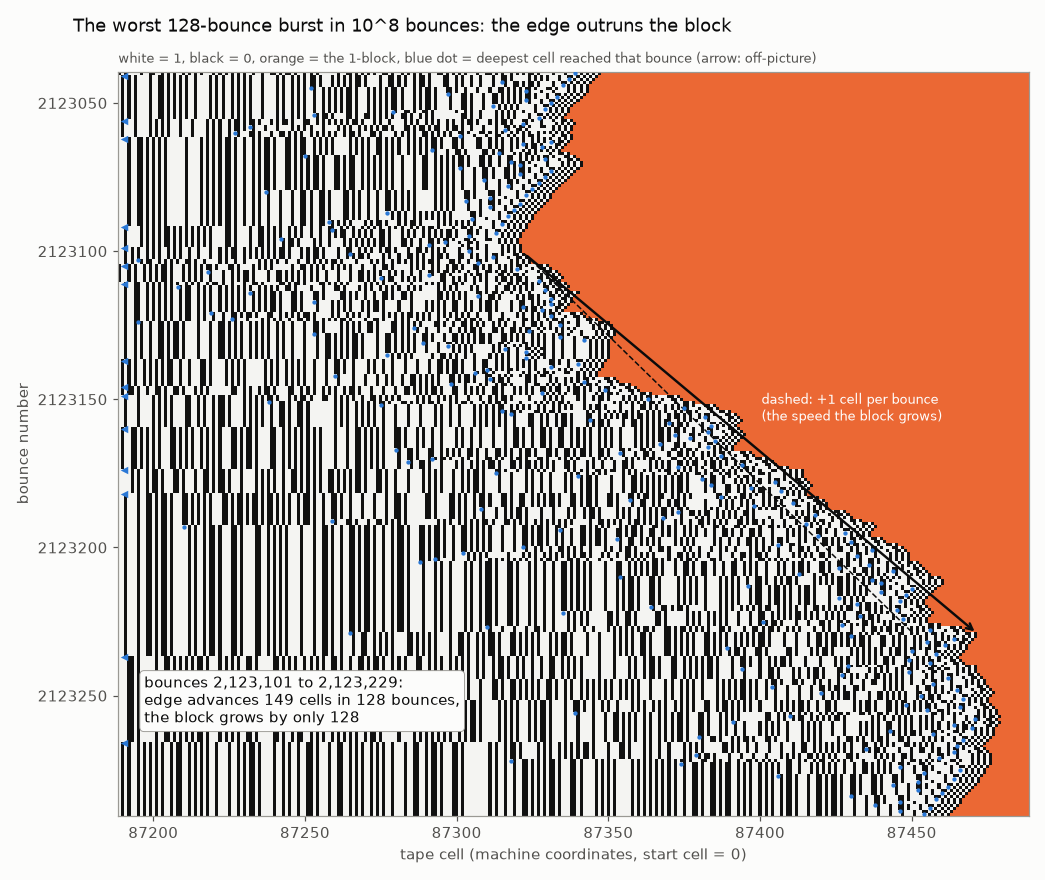
start: mid-run, bounces 2,123,040..2,123,290 (about 4.3·10^12 steps) · rows: one row per bounce: the tape when A reaches the right end · window: cells 87,189..87,488, one pixel column per cell · legend: white = 1, black = 0, orange = the 1-block, blue dot = deepest cell the head reached in that bounce (arrow at the left edge = deeper than shown); the dashed line has slope +1 cell per bounce · style: custom
The diagonal checkerboard stripes are receding phases: the edge end moves 1 cell left per bounce while the counter from section 1 ticks. A burst follows when a deep dive reorganizes the material.
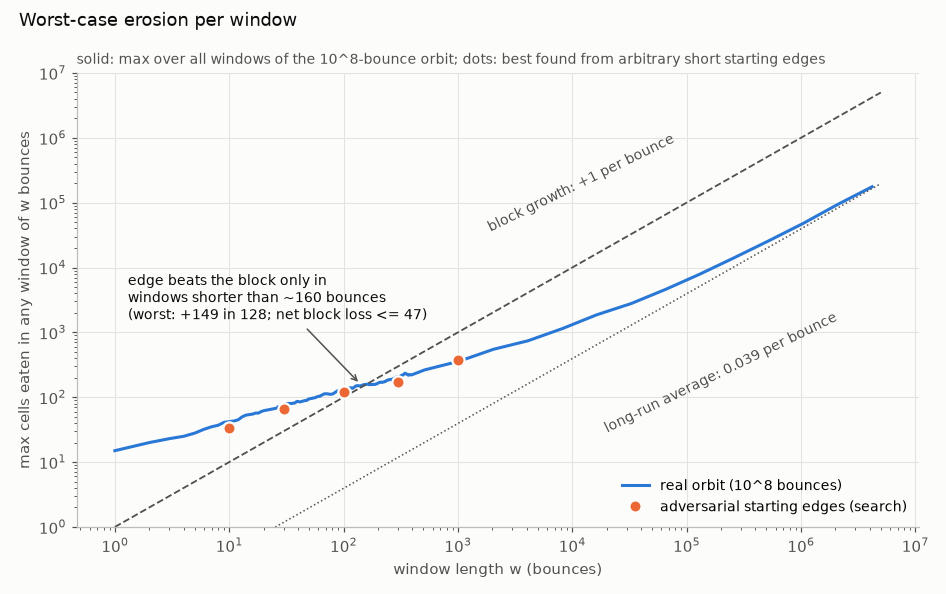
rows/window: n/a (a chart) · legend: blue = max over all windows of the 10^8-bounce orbit; orange dots = best found from arbitrary short starting edges (section 6); dashed = block growth; dotted = long-run average · style: custom chart
| window w (bounces) | 1 | 8 | 32 | 64 | 128 | 160 | 256 | 1,024 | 4,096 |
|---|---|---|---|---|---|---|---|---|---|
| max cells eaten | 15 | 37 | 79 | 107 | 149 | 159 | 187 | 359 | 742 |
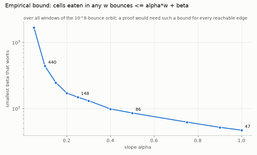
The bound a proof would need, measured on the 10^8-bounce orbit: cells eaten in any w consecutive bounces ≤ α·w + β. The smallest β that works for each slope α:
| α | 0.10 | 0.25 | 0.50 | 1.00 |
|---|---|---|---|---|
| smallest β that works | 441 | 149 | 86 | 47 |
Read-off: empirically, eaten ≤ 0.25·w + 149. A proof needs some such bound for every reachable edge, not just along one orbit.
4. Where erosion comes from: deep dives
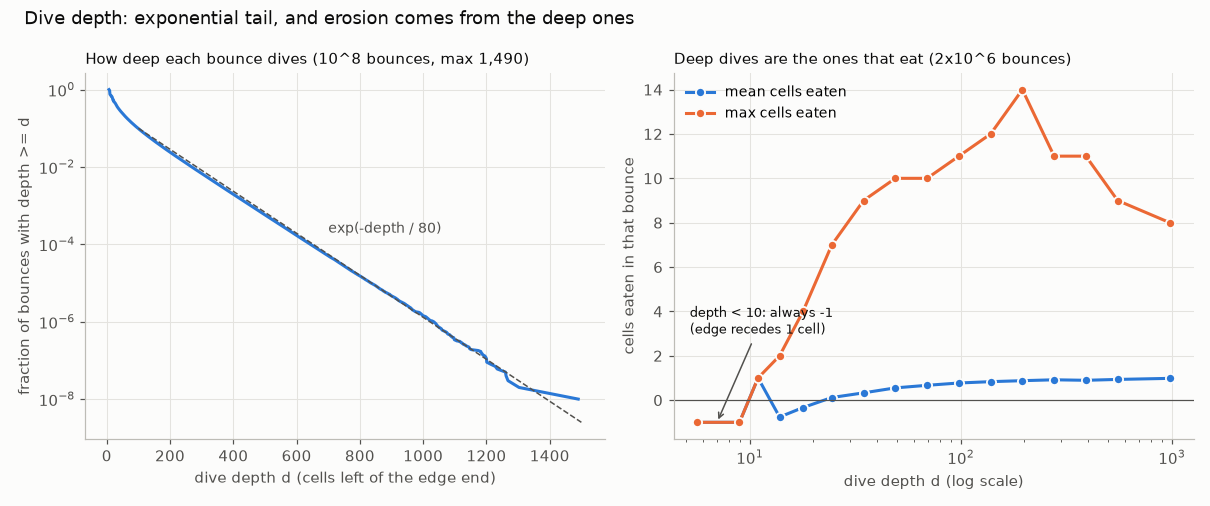
legend (left): fraction of bounces whose dive reaches depth ≥ d, from 10^8 bounces, with the dashed fit exp(−d/80) · legend (right): mean (blue) and max (orange) cells eaten per bounce, by dive depth, from 2·10^6 bounces · style: custom chart
- Depth tail: exponential with scale about 80 cells. The deepest of 10^8 dives was 1,490.
- Shallow bounces are rigid on reachable edges:
- depth < 10 → always −1 (the edge recedes 1 cell);
- depth 10 to 11 → always +1.
- But that depends on reachability: on arbitrary 16-cell tails the same shallow depths allow up to +5 to +7 (exhaustive over 2^15 tails,
code/shallow.py). Even the simplest local fact needs the reachable language.
5. Potential-function search (task item 2)
The goal is a Φ(w) ≥ 0 (or ≥ −γ|w| with γ < 1) with eaten + ΔΦ ≤ α < 1 on every bounce. That would give eaten(k bounces) ≤ α·k + Φ(start). Each family was solved as a linear program over the real orbit.
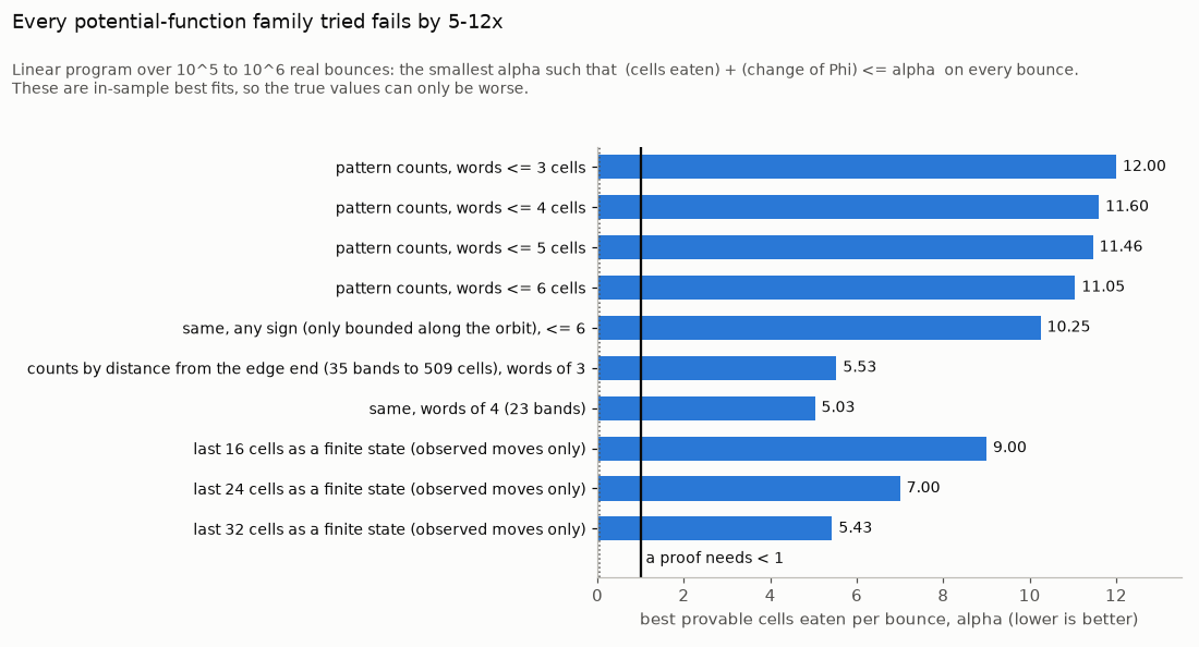
| family (Φ is a linear combination of ...) | orbit sample | best α (need < 1) |
|---|---|---|
| counts of all words ≤ 3/4/5/6 cells in w, plus any bounded term on the last 6 cells | first 10^9 steps (32,222 bounces) | 9.39 / 9.16 / 8.99 / 8.56 |
| same | 10^6 bounces | 12.0 / 11.60 / 11.46 / 11.05 |
| same, any sign (only required bounded along the orbit) | 10^6 bounces | 11.23 / 10.77 / 10.48 / 10.25 |
| counts by distance from the edge end (bounded, any sign): 3-words in 7 or 35 bands, 4-words in 23 bands, out to 509 cells | 10^5 training bounces | 7.08 / 5.53 / 5.03 in-sample (9.4 to 10.1 on the next 10^5) |
| last K cells as a finite state, observed transitions only (optimistic: unsound) | 10^6 bounces | K ≤ 14: 12 · 16: 9 · 20: 7.9 · 24: 7.0 · 32: 5.4 |
| exact conserved local valuation (ΔVal = 1 every bounce, words ≤ 6) | 2.7·10^5 distinct bounces | none (rms residual 0.8) |
Why count potentials cannot work. The LP's dual gives a concrete obstruction. Take the run up to step 10^9 and words of ≤ 4 cells. The dual is a mix of 6 real bounces, each eating 8 to 11 cells: - their end-of-edge states form a closed cycle; - their combined change in every pattern count is ≥ 0.
So after them, any count-based Φ is at least as large as before, while about 9 cells per bounce were eaten. In other words, some bursts create exactly the patterns other bursts destroy. The "fuel" for erosion is not a local statistic (code/dual.py).
How deep the information sits. We computed the ideal potential Φ*(w) = max over the future of (eaten − 0.5·bounces) along the orbit. Then we grouped bounces that share the same last D cells:
| D (cells) | 32 | 48 | 64 |
|---|---|---|---|
| mean spread of Φ* within a group | 37 | 12.4 | 4.1 |
| max spread of Φ* within a group | 85.5 | 84.5 | 84.5 |
So the last 64 cells still do not determine how much the edge will eat; 84.5 is the whole range of Φ*.
6. Regular-language (CTL-style) search (task item 3)
- Factor closures are not invariant. X_m is the set of words all of whose m-cell factors occur in the real edge. Under one bounce, random X_m words leave X_m:
| m | 6 | 8 | 10 | 12 | 14 | 16 | 20 |
|---|---|---|---|---|---|---|---|
| words leaving X_m | 11% | 1.7% | 9% | 11% | 16% | 21% | 29% |
None is closed.
- Not a finite-type language at small scale. The real edge (3.9 million cells) avoids 000, 00100, 001100, 001111 and 0011100. After that the number of minimal forbidden words keeps growing (lengths 9 to 16: 6, 10, 9, 15, 42, 77, 99, 166). Factor counts grow ×1.55 per cell, which is about 0.63 bits of entropy per cell.
- A positive-entropy edge is not substitutive or automatic (those have linear factor complexity). That rules out the usual "renormalize by a substitution" proof.
- Weighted-automaton test. We took the max-mean erosion cycle of the right-end abstraction. Even using only the transitions actually observed, which is an optimistic bound, it gives ≥ 5.4 cells per bounce for windows up to 32 cells (section 5). A sound abstraction contains those cycles too.
7. Is the slow drift universal? (random and adversarial starts)
The wall model was run from starting edges other than the real one:
| starting edges | bounces | result |
|---|---|---|
| 6 uniform-random + 6 random golden-mean words, 200 or 2,000 cells | 10^5 | rate 0.033 to 0.050; worst 100-window 84 to 102; worst 1,000-window 197 to 304 |
| all 226 periodic words with primitive period ≤ 10 (about 1,200 cells) | 2·10^4 | no halt; worst 100-window ≤ 116; at most 235 cells in the first 1,000 bounces |
| every word ≤ 20 cells (exhaustive) | 10 | at most 34 cells |
| every word ≤ 18 cells (exhaustive) | 100 | at most 66 cells |
| hill-climbed words, 30 to 240 cells (adversarial search) | 30 / 100 / 300 / 1,000 | best 66 / 120 / 171 / 373 cells |
| single bounce, every word ≤ 28 cells | 1 | max eaten grows with length: 10 at 15 cells, 17 at 26 and 28 cells |
- No start sustains rate ≥ 1 beyond about 150 bounces. Every start relaxes to the same front (rate ~0.04).
- But per-bounce erosion is unbounded over arbitrary words (it grows with word length). So any bound must use what the reachable edges look like, and section 6 shows that structure is not a small regular language.
8. What is proven, what is empirical, and the best remaining route
| statement | status |
|---|---|
| 7 rules (section 1) and their completeness under the no-00 invariant | proven by case analysis + sim 60/60 each |
| dive = binary-counter carry on parities of every other run | proven by induction from Ca/Fo/T + 15,450/15,450 check |
| wall model exact while n ≥ e + 3 | argument + per-bounce check |
| no halt in the first ~9.6·10^15 steps (10^8 bounces) | computation (exact wall model) |
| front speed 0.039 per bounce; eaten ≤ 0.25·w + 149 in every window; block ≥ 33 after bounce 40 | empirical (10^8 bounces) |
| same drift from random, periodic, exhaustive and adversarial starts | empirical |
| no potential from pattern counts (≤ 6-cell words, also by distance bands to 509 cells, also with a 32-cell finite state) gives α < 5 | computed (LP, in-sample, so the real α is worse) |
| a deterministic bound α·k + β with α < 1 | open; no route found |
Most promising (still long-shot) proof route: a two-scale computer-assisted abstraction.
- State: - the exact last D cells of the edge; - a sound regular summary of the deep part.
The rules make this possible in principle: the head enters the deep part only as a C dive and comes back only as an A return. So a deep excursion is a black box with few possible effects on the window. 2. Invariant: find a regular language for the deep part that rules out the adversarial returns. 3. Check: compute the max-mean-cycle erosion of the finite product graph and show it is < 1.
Measured obstacles: - Windows up to D = 32 already contain cycles eating 5.4 per bounce, so D must be well above 64. - Distinct reachable tails grow about ×1.35 per cell: 58,000 at D = 40 in only 4·10^5 bounces. That points to 10^12 or more states at D = 100. - Small factor-closed deep languages are not invariant.
Without a new compression idea this is out of reach. A hidden-arithmetic route (the edge as a counter in some numeration) is unlikely: there is no conserved local valuation, the entropy is positive, and the counter structure lasts only 2 to 3 levels before the deep part turns pseudo-random.
Bottom line for Dennis: #5 halting reduces to "a chaotic front never outruns a block that grows 25× faster on average". That is true over 10^16 steps by a wide margin, but proving it looks as hard as a cryptid.
Reproduce
Code is in research/code/. It was run from the session scratchpad, so paths inside it point there.
| file | what it does |
|---|---|
wallc.c |
wall-model runner: per-bounce eaten and depth, window maxima, snapshots, range dumps |
phistar.c |
α to β curve (smallest β per slope) |
feat.c, lp.py, lp2.py, band.py, tailmmc.py, conserve.py, dual.py |
potential searches |
locality.py |
the Φ* spread test |
sftinv2.py, mfw.py |
regular-language tests |
wallmany.c, exh1.c, climb.c |
other starting edges |
verify_rules.py, divecheck.py, shallow.py |
rule checks |
fig_*.py, figs.py |
figures |
run_1e8.summary.txt |
the 10^8-bounce summary |